Program
“Complete Example 1” showed how to create a simple demographics table using the fmtr package and Tidyverse. Here is the same table created with only Base R and the sassy system of packages.
The data for this example has been included in the
fmtr package as an external data file. It may be
accessed using the system.file() function as shown below,
or downloaded directly from the fmtr GitHub site here
library(sassy)

# Prepare Log -------------------------------------------------------------


options("logr.autolog" = TRUE,
        "logr.notes" = FALSE)

# Get temp location for log and report output
tmp <- tempdir()

# Open log
lf <- log_open(file.path(tmp, "example2.log"))


# Load and Prepare Data ---------------------------------------------------

sep("Prepare Data")

# Get path to sample data
pkg <- system.file("extdata", package = "fmtr")

# Define data library
libname(sdtm, pkg, "csv")

# Prepare data
put("Subset DM dataset")
dm_mod <- subset(sdtm$DM, ARM != "SCREEN FAILURE",
                 v(USUBJID, SEX, AGE, ARM)) |> put()

put("Get ARM population counts")
arm_pop <- proc_freq(dm_mod, tables = ARM,
                     output = long,
                     options = v(nocum, nopercent, nonobs))


# Create Format Catalog --------------------------------------------------
sep("Create format catalog")

fmts <- fcat(AGECAT = value(condition(x >= 18 & x <= 24, "18 to 24"),
                            condition(x >= 25 & x <= 44, "25 to 44"),
                            condition(x >= 45 & x <= 64, "45 to 64"),
                            condition(x >= 65, ">= 65")),
             SEX = value(condition(is.na(x), "Missing", order = 3),
                         condition(x == "M", "Male", order = 1),
                         condition(x == "F", "Female", order = 2)),
             VAR = c("AGE" = "Age",
                     "AGECAT" = "Age Group",
                     "SEX" = "Sex"))

numfmts <- fcat(N = "%d", MEAN = "%.1f", STD = "(%04.2f)", MEDIAN = "%d", Q1 = "%.1f",
                Q3 = "%.1f", MIN = "%d", MAX = "%d", CNT = "%d", PCT = "(%4.1f%%)")

numlbls <- c(N = "n", MEANSD = "Mean (SD)", MEDIAN = "Median", Q1Q3 = "Q1 - Q3",
             MINMAX = "Min - Max")

# Age Summary Block -------------------------------------------------------

sep("Create summary statistics for age")

age_block <- proc_means(dm_mod, stats = v(n, mean, std, median, q1, q3, min, max),
                        class = ARM, options = v(nway, notype, nofreq)) |>
  datastep(format = numfmts,
           keep = v(CLASS, VAR, N, MEANSD, MEDIAN, Q1Q3, MINMAX),
           {

             MEANSD <- fapply2(MEAN, STD)
             Q1Q3 <- fapply2(Q1, Q3, sep = " - ")
             MINMAX <- fapply2(MIN, MAX, sep = " - ")
           }) |>
  proc_transpose(id = CLASS, copy = VAR,
                 var = v(N, MEANSD, MEDIAN, Q1Q3, MINMAX),
                 name = "LABEL") |>
  datastep({LABEL <- fapply(LABEL, numlbls)})


# Age Group Block ----------------------------------------------------------

sep("Create frequency counts for Age Group")

put("Create age group frequency counts")
ageg_block <- dm_mod |>
  datastep({AGECAT <- fapply(AGE, fmts$AGECAT)}) |>
  proc_freq(tables = AGECAT, by = ARM,
            options = nonobs) |>
  datastep(format = numfmts,
           keep = v(VAR, BY, LABEL, CNTPCT),
           {
             LABEL <- CAT
             CNTPCT <- fapply2(CNT, PCT)
           }) |>
  proc_transpose(var = CNTPCT, by = LABEL, copy = VAR, id = BY, options = noname)

put("Sort age groups as desired")
ageg_block$LABEL <- factor(ageg_block$LABEL, levels = levels(fmts$AGECAT))
ageg_block <- proc_sort(ageg_block, by = LABEL, as.character = TRUE)


# Sex Block ---------------------------------------------------------------

sep("Create frequency counts for SEX")

put("Create sex frequency counts")
sex_block <- dm_mod |>
  datastep({SEX <- fapply(SEX, fmts$SEX)}) |>
  proc_freq(tables = SEX, by = ARM,
            options = nonobs) |>
  datastep(format = numfmts,
           keep = v(VAR, BY, LABEL, CNTPCT),
           {
             LABEL <- CAT
             CNTPCT <- fapply2(CNT, PCT)
           }) |>
  proc_transpose(var = CNTPCT, by = LABEL, copy = VAR, id = BY, options = noname)

put("Sort age groups as desired")
sex_block$LABEL <- factor(sex_block$LABEL, levels = levels(fmts$SEX))
sex_block <- proc_sort(sex_block, by = LABEL, as.character = TRUE)


put("Combine blocks into final data frame")
final <- bind_rows(age_block, ageg_block, sex_block) |> put()

# Report ------------------------------------------------------------------


sep("Create and print report")

# Create Table
tbl <- create_table(final, first_row_blank = TRUE, borders = c("top", "bottom")) |>
  column_defaults(from = `ARM A`, to = `ARM D`, align = "center", width = 1.25) |>
  stub(vars = v(VAR, LABEL), "Variable", width = 2.5) |>
  define(VAR, blank_after = TRUE, dedupe = TRUE, label = "Variable",
         format = fmts$VAR,label_row = TRUE) |>
  define(LABEL, indent = .25, label = "Demographic Category") |>
  define(`ARM A`,  label = "Treatment Group 1", n = arm_pop["ARM A"]) |>
  define(`ARM B`,  label = "Treatment Group 2", n = arm_pop["ARM B"]) |>
  define(`ARM C`,  label = "Treatment Group 3", n = arm_pop["ARM C"]) |>
  define(`ARM D`,  label = "Treatment Group 4", n = arm_pop["ARM D"])

rpt <- create_report(file.path(tmp, "output/example2.rtf"),
                     output_type = "RTF", font = "Arial") |>
  set_margins(top = 1, bottom = 1) |>
  page_header("Sponsor: Company", "Study: ABC") |>
  titles("Table 1.0", bold = TRUE, blank_row = "none") |>
  titles("Analysis of Demographic Characteristics",
         "Safety Population") |>
  add_content(tbl) |>
  footnotes("Program: DM_Table.R",
            "NOTE: Denominator based on number of non-missing responses.") |>
  page_footer(paste0("Date Produced: ", fapply(Sys.time(), "%d%b%y %H:%M")),
              right = "Page [pg] of [tpg]")

res <- write_report(rpt)


# Clean Up ----------------------------------------------------------------
sep("Clean Up")

# Close log
log_close()

# View report
# file.show(res$modified_path)

# View log
# file.show(lf)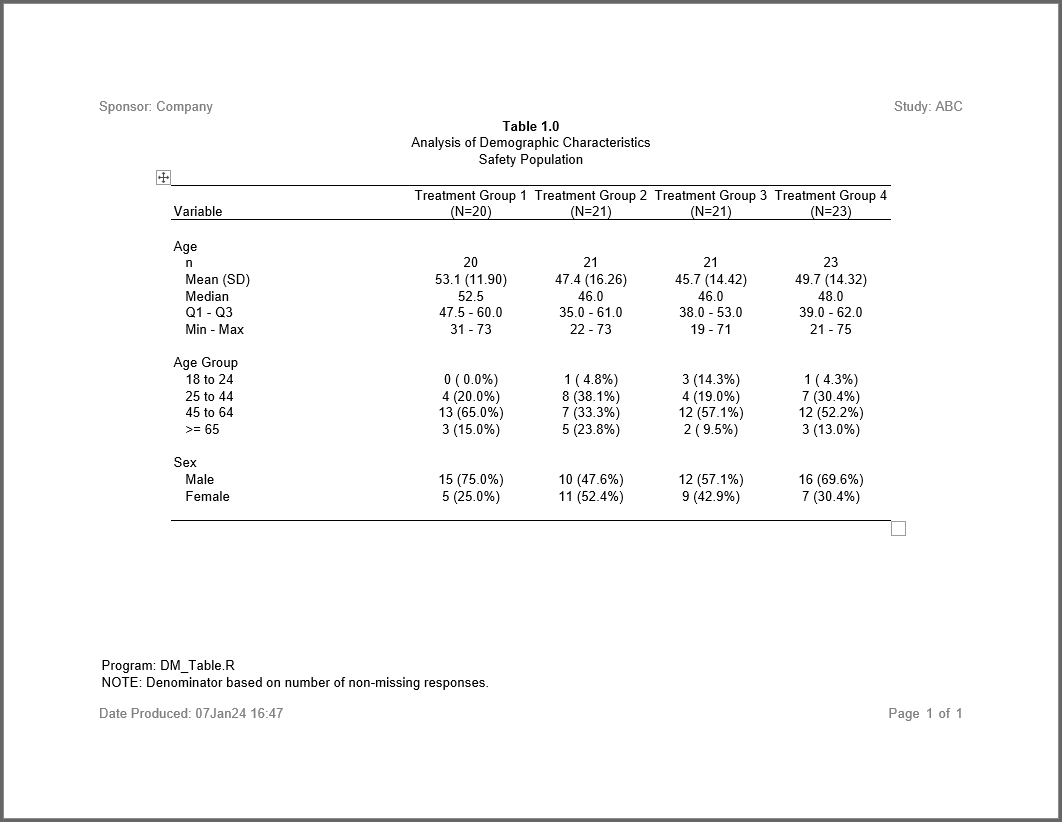
Log
Here is the log produced by the above sample program:
=========================================================================
Log Path: C:/Users/dbosa/AppData/Local/Temp/RtmpKc23Rz/log/example2.log
Program Path: C:/Users/dbosa/Documents/.active-rstudio-document
Working Directory: C:/Projects/Archytas/Sassy/Code
User Name: dbosa
R Version: 4.3.2 (2023-10-31 ucrt)
Machine: SOCRATES x86-64
Operating System: Windows 10 x64 build 22621
Base Packages: stats graphics grDevices utils datasets methods base Other
Packages: tidylog_1.0.2 reporter_1.4.4 logr_1.3.5 sassy_1.2.1 lubridate_1.9.2
forcats_1.0.0 stringr_1.5.0 purrr_1.0.1 readr_2.1.4 tidyr_1.3.0 tibble_3.2.1
ggplot2_3.4.4 tidyverse_2.0.0 libr_1.2.8 dplyr_1.1.3 fmtr_1.6.2 procs_1.0.4
common_1.1.1
Log Start Time: 2024-01-07 18:26:25.636328
=========================================================================

=========================================================================
Prepare Data
=========================================================================

# library 'sdtm': 1 items
- attributes: csv not loaded
- path: C:/Users/dbosa/AppData/Local/R/win-library/4.3/fmtr/extdata
- items:
  Name Extension Rows Cols    Size        LastModified
1   DM       csv   87   24 45.5 Kb 2023-12-16 23:10:51

Subset DM dataset

# A tibble: 85 × 4
   USUBJID    SEX     AGE ARM
   <chr>      <chr> <dbl> <chr>
 1 ABC-01-049 M        39 ARM D
 2 ABC-01-050 M        47 ARM B
 3 ABC-01-051 M        34 ARM A
 4 ABC-01-052 F        45 ARM C
 5 ABC-01-053 F        26 ARM B
 6 ABC-01-054 M        44 ARM D
 7 ABC-01-055 F        47 ARM C
 8 ABC-01-056 M        31 ARM A
 9 ABC-01-113 M        74 ARM D
10 ABC-01-114 F        72 ARM B
# ℹ 75 more rows
# ℹ Use `print(n = ...)` to see more rows

Get ARM population counts

proc_freq: input data set 85 rows and 4 columns
           tables: ARM
           output: long
           view: TRUE
           output: 1 datasets

# A tibble: 1 × 6
  VAR   STAT  `ARM A` `ARM B` `ARM C` `ARM D`
  <chr> <chr>   <dbl>   <dbl>   <dbl>   <dbl>
1 ARM   CNT        20      21      21      23

=========================================================================
Create format catalog
=========================================================================

# A user-defined format: 4 conditions
  Name Type        Expression    Label Order
1  obj    U x >= 18 & x <= 24 18 to 24    NA
2  obj    U x >= 25 & x <= 44 25 to 44    NA
3  obj    U x >= 45 & x <= 64 45 to 64    NA
4  obj    U           x >= 65    >= 65    NA

# A user-defined format: 3 conditions
  Name Type Expression   Label Order
1  obj    U   is.na(x) Missing     3
2  obj    U   x == "M"    Male     1
3  obj    U   x == "F"  Female     2

# A format catalog: 3 formats
- $AGECAT: type U, 4 conditions
- $SEX: type U, 3 conditions
- $VAR: type V, 3 elements

# A format catalog: 10 formats
- $N: type S, "%d"
- $MEAN: type S, "%.1f"
- $STD: type S, "(%04.2f)"
- $MEDIAN: type S, "%d"
- $Q1: type S, "%.1f"
- $Q3: type S, "%.1f"
- $MIN: type S, "%d"
- $MAX: type S, "%d"
- $CNT: type S, "%d"
- $PCT: type S, "(%4.1f%%)"

=========================================================================
Create summary statistics for age
=========================================================================

proc_means: input data set 85 rows and 4 columns
            class: ARM
            var: AGE
            stats: n mean std median q1 q3 min max
            view: TRUE
            output: 1 datasets

  CLASS VAR  N     MEAN      STD MEDIAN   Q1 Q3 MIN MAX
1 ARM A AGE 20 53.15000 11.89991   52.5 47.5 60  31  73
2 ARM B AGE 21 47.38095 16.25877   46.0 35.0 61  22  73
3 ARM C AGE 21 45.71429 14.41923   46.0 38.0 53  19  71
4 ARM D AGE 23 49.73913 14.32486   48.0 39.0 62  21  75

datastep: columns decreased from 10 to 7

  CLASS VAR  N       MEANSD MEDIAN        Q1Q3  MINMAX
1 ARM A AGE 20 53.1 (11.90)   52.5 47.5 - 60.0 31 - 73
2 ARM B AGE 21 47.4 (16.26)   46.0 35.0 - 61.0 22 - 73
3 ARM C AGE 21 45.7 (14.42)   46.0 38.0 - 53.0 19 - 71
4 ARM D AGE 23 49.7 (14.32)   48.0 39.0 - 62.0 21 - 75

proc_transpose: input data set 4 rows and 7 columns
                var: N MEANSD MEDIAN Q1Q3 MINMAX
                id: CLASS
                copy: VAR
                name: LABEL
                output dataset 5 rows and 6 columns

  VAR  LABEL        ARM A        ARM B        ARM C        ARM D
1 AGE      N           20           21           21           23
2 AGE MEANSD 53.1 (11.90) 47.4 (16.26) 45.7 (14.42) 49.7 (14.32)
3 AGE MEDIAN         52.5         46.0         46.0         48.0
4 AGE   Q1Q3  47.5 - 60.0  35.0 - 61.0  38.0 - 53.0  39.0 - 62.0
5 AGE MINMAX      31 - 73      22 - 73      19 - 71      21 - 75

datastep: columns started with 6 and ended with 6

  VAR     LABEL        ARM A        ARM B        ARM C        ARM D
1 AGE         n           20           21           21           23
2 AGE Mean (SD) 53.1 (11.90) 47.4 (16.26) 45.7 (14.42) 49.7 (14.32)
3 AGE    Median         52.5         46.0         46.0         48.0
4 AGE   Q1 - Q3  47.5 - 60.0  35.0 - 61.0  38.0 - 53.0  39.0 - 62.0
5 AGE Min - Max      31 - 73      22 - 73      19 - 71      21 - 75

=========================================================================
Create frequency counts for Age Group
=========================================================================

Create age group frequency counts

datastep: columns increased from 4 to 5

# A tibble: 85 × 5
   USUBJID    SEX     AGE ARM   AGECAT
   <chr>      <chr> <dbl> <chr> <chr>
 1 ABC-01-049 M        39 ARM D 25 to 44
 2 ABC-01-050 M        47 ARM B 45 to 64
 3 ABC-01-051 M        34 ARM A 25 to 44
 4 ABC-01-052 F        45 ARM C 45 to 64
 5 ABC-01-053 F        26 ARM B 25 to 44
 6 ABC-01-054 M        44 ARM D 25 to 44
 7 ABC-01-055 F        47 ARM C 45 to 64
 8 ABC-01-056 M        31 ARM A 25 to 44
 9 ABC-01-113 M        74 ARM D >= 65
10 ABC-01-114 F        72 ARM B >= 65
# ℹ 75 more rows
# ℹ Use `print(n = ...)` to see more rows

proc_freq: input data set 85 rows and 5 columns
           tables: AGECAT
           by: ARM
           view: TRUE
           output: 1 datasets

# A tibble: 16 × 5
   BY    VAR    CAT        CNT   PCT
   <chr> <chr>  <chr>    <dbl> <dbl>
 1 ARM A AGECAT >= 65        3 15
 2 ARM A AGECAT 18 to 24     0  0
 3 ARM A AGECAT 25 to 44     4 20
 4 ARM A AGECAT 45 to 64    13 65
 5 ARM B AGECAT >= 65        5 23.8
 6 ARM B AGECAT 18 to 24     1  4.76
 7 ARM B AGECAT 25 to 44     8 38.1
 8 ARM B AGECAT 45 to 64     7 33.3
 9 ARM C AGECAT >= 65        2  9.52
10 ARM C AGECAT 18 to 24     3 14.3
11 ARM C AGECAT 25 to 44     4 19.0
12 ARM C AGECAT 45 to 64    12 57.1
13 ARM D AGECAT >= 65        3 13.0
14 ARM D AGECAT 18 to 24     1  4.35
15 ARM D AGECAT 25 to 44     7 30.4
16 ARM D AGECAT 45 to 64    12 52.2

datastep: columns decreased from 5 to 4

# A tibble: 16 × 4
   VAR    BY    LABEL    CNTPCT
   <chr>  <chr> <chr>    <chr>
 1 AGECAT ARM A >= 65    3 (15.0%)
 2 AGECAT ARM A 18 to 24 0 ( 0.0%)
 3 AGECAT ARM A 25 to 44 4 (20.0%)
 4 AGECAT ARM A 45 to 64 13 (65.0%)
 5 AGECAT ARM B >= 65    5 (23.8%)
 6 AGECAT ARM B 18 to 24 1 ( 4.8%)
 7 AGECAT ARM B 25 to 44 8 (38.1%)
 8 AGECAT ARM B 45 to 64 7 (33.3%)
 9 AGECAT ARM C >= 65    2 ( 9.5%)
10 AGECAT ARM C 18 to 24 3 (14.3%)
11 AGECAT ARM C 25 to 44 4 (19.0%)
12 AGECAT ARM C 45 to 64 12 (57.1%)
13 AGECAT ARM D >= 65    3 (13.0%)
14 AGECAT ARM D 18 to 24 1 ( 4.3%)
15 AGECAT ARM D 25 to 44 7 (30.4%)
16 AGECAT ARM D 45 to 64 12 (52.2%)

proc_transpose: input data set 16 rows and 4 columns
                by: LABEL
                var: CNTPCT
                id: BY
                copy: VAR
                name: NAME
                output dataset 4 rows and 6 columns

# A tibble: 4 × 6
  VAR    LABEL    `ARM A`    `ARM B`   `ARM C`    `ARM D`
  <chr>  <chr>    <chr>      <chr>     <chr>      <chr>
1 AGECAT >= 65    3 (15.0%)  5 (23.8%) 2 ( 9.5%)  3 (13.0%)
2 AGECAT 18 to 24 0 ( 0.0%)  1 ( 4.8%) 3 (14.3%)  1 ( 4.3%)
3 AGECAT 25 to 44 4 (20.0%)  8 (38.1%) 4 (19.0%)  7 (30.4%)
4 AGECAT 45 to 64 13 (65.0%) 7 (33.3%) 12 (57.1%) 12 (52.2%)

Sort age groups as desired

proc_sort: input data set 4 rows and 6 columns
           by: LABEL
           keep: VAR LABEL ARM A ARM B ARM C ARM D
           order: a
           output data set 4 rows and 6 columns

# A tibble: 4 × 6
  VAR    LABEL    `ARM A`    `ARM B`   `ARM C`    `ARM D`
  <chr>  <chr>    <chr>      <chr>     <chr>      <chr>
1 AGECAT 18 to 24 0 ( 0.0%)  1 ( 4.8%) 3 (14.3%)  1 ( 4.3%)
2 AGECAT 25 to 44 4 (20.0%)  8 (38.1%) 4 (19.0%)  7 (30.4%)
3 AGECAT 45 to 64 13 (65.0%) 7 (33.3%) 12 (57.1%) 12 (52.2%)
4 AGECAT >= 65    3 (15.0%)  5 (23.8%) 2 ( 9.5%)  3 (13.0%)

=========================================================================
Create frequency counts for SEX
=========================================================================

Create sex frequency counts

datastep: columns started with 4 and ended with 4

# A tibble: 85 × 4
   USUBJID    SEX      AGE ARM
   <chr>      <chr>  <dbl> <chr>
 1 ABC-01-049 Male      39 ARM D
 2 ABC-01-050 Male      47 ARM B
 3 ABC-01-051 Male      34 ARM A
 4 ABC-01-052 Female    45 ARM C
 5 ABC-01-053 Female    26 ARM B
 6 ABC-01-054 Male      44 ARM D
 7 ABC-01-055 Female    47 ARM C
 8 ABC-01-056 Male      31 ARM A
 9 ABC-01-113 Male      74 ARM D
10 ABC-01-114 Female    72 ARM B
# ℹ 75 more rows
# ℹ Use `print(n = ...)` to see more rows

proc_freq: input data set 85 rows and 4 columns
           tables: SEX
           by: ARM
           view: TRUE
           output: 1 datasets

# A tibble: 8 × 5
  BY    VAR   CAT      CNT   PCT
  <chr> <chr> <chr>  <dbl> <dbl>
1 ARM A SEX   Female     5  25
2 ARM A SEX   Male      15  75
3 ARM B SEX   Female    11  52.4
4 ARM B SEX   Male      10  47.6
5 ARM C SEX   Female     9  42.9
6 ARM C SEX   Male      12  57.1
7 ARM D SEX   Female     7  30.4
8 ARM D SEX   Male      16  69.6

datastep: columns decreased from 5 to 4

# A tibble: 8 × 4
  VAR   BY    LABEL  CNTPCT
  <chr> <chr> <chr>  <chr>
1 SEX   ARM A Female 5 (25.0%)
2 SEX   ARM A Male   15 (75.0%)
3 SEX   ARM B Female 11 (52.4%)
4 SEX   ARM B Male   10 (47.6%)
5 SEX   ARM C Female 9 (42.9%)
6 SEX   ARM C Male   12 (57.1%)
7 SEX   ARM D Female 7 (30.4%)
8 SEX   ARM D Male   16 (69.6%)

proc_transpose: input data set 8 rows and 4 columns
                by: LABEL
                var: CNTPCT
                id: BY
                copy: VAR
                name: NAME
                output dataset 2 rows and 6 columns

# A tibble: 2 × 6
  VAR   LABEL  `ARM A`    `ARM B`    `ARM C`    `ARM D`
  <chr> <chr>  <chr>      <chr>      <chr>      <chr>
1 SEX   Female 5 (25.0%)  11 (52.4%) 9 (42.9%)  7 (30.4%)
2 SEX   Male   15 (75.0%) 10 (47.6%) 12 (57.1%) 16 (69.6%)

Sort age groups as desired

proc_sort: input data set 2 rows and 6 columns
           by: LABEL
           keep: VAR LABEL ARM A ARM B ARM C ARM D
           order: a
           output data set 2 rows and 6 columns

# A tibble: 2 × 6
  VAR   LABEL  `ARM A`    `ARM B`    `ARM C`    `ARM D`
  <chr> <chr>  <chr>      <chr>      <chr>      <chr>
1 SEX   Male   15 (75.0%) 10 (47.6%) 12 (57.1%) 16 (69.6%)
2 SEX   Female 5 (25.0%)  11 (52.4%) 9 (42.9%)  7 (30.4%)

Combine blocks into final data frame

      VAR     LABEL        ARM A        ARM B        ARM C        ARM D
1     AGE         n           20           21           21           23
2     AGE Mean (SD) 53.1 (11.90) 47.4 (16.26) 45.7 (14.42) 49.7 (14.32)
3     AGE    Median         52.5         46.0         46.0         48.0
4     AGE   Q1 - Q3  47.5 - 60.0  35.0 - 61.0  38.0 - 53.0  39.0 - 62.0
5     AGE Min - Max      31 - 73      22 - 73      19 - 71      21 - 75
6  AGECAT  18 to 24    0 ( 0.0%)    1 ( 4.8%)    3 (14.3%)    1 ( 4.3%)
7  AGECAT  25 to 44    4 (20.0%)    8 (38.1%)    4 (19.0%)    7 (30.4%)
8  AGECAT  45 to 64   13 (65.0%)    7 (33.3%)   12 (57.1%)   12 (52.2%)
9  AGECAT     >= 65    3 (15.0%)    5 (23.8%)    2 ( 9.5%)    3 (13.0%)
10    SEX      Male   15 (75.0%)   10 (47.6%)   12 (57.1%)   16 (69.6%)
11    SEX    Female    5 (25.0%)   11 (52.4%)    9 (42.9%)    7 (30.4%)

=========================================================================
Create and print report
=========================================================================

# A report specification: 1 pages
- file_path: 'C:\Users\dbosa\AppData\Local\Temp\RtmpKc23Rz/output/example2.rtf'
- output_type: RTF
- units: inches
- orientation: landscape
- margins: top 1 bottom 1 left 1 right 1
- line size/count: 9/36
- page_header: left=Sponsor: Company right=Study: ABC
- title 1: 'Table 1.0'
- title 2: 'Analysis of Demographic Characteristics'
- title 3: 'Safety Population'
- footnote 1: 'Program: DM_Table.R'
- footnote 2: 'NOTE: Denominator based on number of non-missing responses.'
- page_footer: left=Date Produced: 07Jan24 18:26 center= right=Page [pg] of [tpg]
- content:
# A table specification:
- data: data.frame 'final' 11 rows 6 cols
- show_cols: all
- use_attributes: all
- stub: VAR LABEL 'Variable' width=2.5 align='left'
- define: VAR 'Variable' dedupe='TRUE'
- define: LABEL 'Demographic Category'
- define: ARM A 'Treatment Group 1'
- define: ARM B 'Treatment Group 2'
- define: ARM C 'Treatment Group 3'
- define: ARM D 'Treatment Group 4'

=========================================================================
Clean Up
=========================================================================

=========================================================================
Log End Time: 2024-01-07 18:26:27.426253
Log Elapsed Time: 0 00:00:01
=========================================================================