Program
The previous examples in the fmtr documentation were intentionally simplified to focus on the workings of a particular function. It is helpful to also view fmtr functions in the context of a complete program. The following example shows a complete program.
The data for this example has been included in the
fmtr package as an external data file. It may be
accessed using the system.file() function as shown below,
or downloaded directly from the fmtr GitHub site here
library(tidyverse)
library(sassy)


# Prepare Log -------------------------------------------------------------


options("logr.autolog" = TRUE,
        "logr.notes" = FALSE)

# Get temp location for log and report output
tmp <- tempdir()

# Open log
lf <- log_open(file.path(tmp, "example1.log"))


# Load and Prepare Data ---------------------------------------------------

sep("Prepare Data")

# Get path to sample data
pkg <- system.file("extdata", package = "fmtr")

# Define data library
libname(sdtm, pkg, "csv")

# Prepare data
dm_mod <- sdtm$DM %>%
  select(USUBJID, SEX, AGE, ARM) %>%
  filter(ARM != "SCREEN FAILURE") %>%
  put()


put("Get ARM population counts")
arm_pop <- count(dm_mod, ARM) %>% deframe() %>% put()

# Create Format Catalog --------------------------------------------------
sep("Create format catalog")

fmts <- fcat(AGECAT = value(condition(x >= 18 & x <= 24, "18 to 24"),
                            condition(x >= 25 & x <= 44, "25 to 44"),
                            condition(x >= 45 & x <= 64, "45 to 64"),
                            condition(x >= 65, ">= 65"),
                            condition(TRUE, "Other")),
             SEX = value(condition(is.na(x), "Missing"),
                         condition(x == "M", "Male"),
                         condition(x == "F", "Female"),
                         condition(TRUE, "Other")),
             VAR = c("AGE" = "Age",
                     "AGECAT" = "Age Group",
                     "SEX" = "Sex"))
put(fmts)

# Age Summary Block -------------------------------------------------------

sep("Create summary statistics for age")

age_block <-
  dm_mod %>%
  group_by(ARM) %>%
  summarise( N = fmt_n(AGE),
             `Mean (SD)` = fmt_mean_sd(AGE),
             Median = fmt_median(AGE),
             `Q1 - Q3` = fmt_quantile_range(AGE),
             Range  = fmt_range(AGE)) %>%
  pivot_longer(-ARM,
               names_to  = "label",
               values_to = "value") %>%
  pivot_wider(names_from = ARM,
              values_from = "value") %>%
  add_column(var = "AGE", .before = "label") %>%
  put()


# Age Group Block ----------------------------------------------------------

sep("Create frequency counts for Age Group")


put("Create age group frequency counts")
ageg_block <-
  dm_mod %>%
  mutate(AGECAT = fapply(AGE, fmts$AGECAT)) %>%
  select(ARM, AGECAT) %>%
  group_by(ARM, AGECAT) %>%
  summarize(n = n()) %>%
  pivot_wider(names_from = ARM,
              values_from = n,
              values_fill = 0) %>%
  transmute(var = "AGECAT",
            label =  factor(AGECAT, levels = c("18 to 24",
                                               "25 to 44",
                                               "45 to 64",
                                               ">= 65")),
            `ARM A` = fmt_cnt_pct(`ARM A`, arm_pop["ARM A"]),
            `ARM B` = fmt_cnt_pct(`ARM B`, arm_pop["ARM B"]),
            `ARM C` = fmt_cnt_pct(`ARM C`, arm_pop["ARM C"]),
            `ARM D` = fmt_cnt_pct(`ARM D`, arm_pop["ARM D"])) %>%
  arrange(label) %>%
  put()


# Sex Block ---------------------------------------------------------------

sep("Create frequency counts for SEX")


# Create sex frequency counts
sex_block <-
  dm_mod %>%
  select(ARM, SEX) %>%
  group_by(ARM, SEX) %>%
  summarize(n = n()) %>%
  pivot_wider(names_from = ARM,
              values_from = n,
              values_fill = 0) %>%
  transmute(var = "SEX",
            label =   fct_relevel(SEX, "M", "F"),
            `ARM A` = fmt_cnt_pct(`ARM A`, arm_pop["ARM A"]),
            `ARM B` = fmt_cnt_pct(`ARM B`, arm_pop["ARM B"]),
            `ARM C` = fmt_cnt_pct(`ARM C`, arm_pop["ARM C"]),
            `ARM D` = fmt_cnt_pct(`ARM D`, arm_pop["ARM D"])) %>%
  arrange(label) %>%
  mutate(label = fapply(label, fmts$SEX)) %>%
  put()

put("Combine blocks into final data frame")
final <- bind_rows(age_block, ageg_block, sex_block) %>% put()

# Report ------------------------------------------------------------------


sep("Create and print report")


# Create Table
tbl <- create_table(final, first_row_blank = TRUE, borders = c("top", "bottom")) %>%
  column_defaults(from = `ARM A`, to = `ARM D`, align = "center", width = 1.25) %>%
  stub(vars = c("var", "label"), "Variable", width = 2.5) %>%
  define(var, blank_after = TRUE, dedupe = TRUE, label = "Variable",
         format = fmts$VAR,label_row = TRUE) %>%
  define(label, indent = .25, label = "Demographic Category") %>%
  define(`ARM A`,  label = "Treatment Group 1", n = arm_pop["ARM A"]) %>%
  define(`ARM B`,  label = "Treatment Group 2", n = arm_pop["ARM B"]) %>%
  define(`ARM C`,  label = "Treatment Group 3", n = arm_pop["ARM C"]) %>%
  define(`ARM D`,  label = "Treatment Group 4", n = arm_pop["ARM D"])

rpt <- create_report(file.path(tmp, "output/example1.rtf"),
                     output_type = "RTF", font = "Arial") %>%
  set_margins(top = 1, bottom = 1) %>%
  page_header("Sponsor: Company", "Study: ABC") %>%
  titles("Table 1.0", bold = TRUE, blank_row = "none") %>%
  titles("Analysis of Demographic Characteristics",
         "Safety Population") %>%
  add_content(tbl) %>%
  footnotes("Program: DM_Table.R",
            "NOTE: Denominator based on number of non-missing responses.") %>%
  page_footer(paste0("Date Produced: ", fapply(Sys.time(), "%d%b%y %H:%M")),
              right = "Page [pg] of [tpg]")

res <- write_report(rpt)


# Clean Up ----------------------------------------------------------------
sep("Clean Up")

# Close log
log_close()

# View report
# file.show(res$modified_path)

# View Log
# file.show(lf)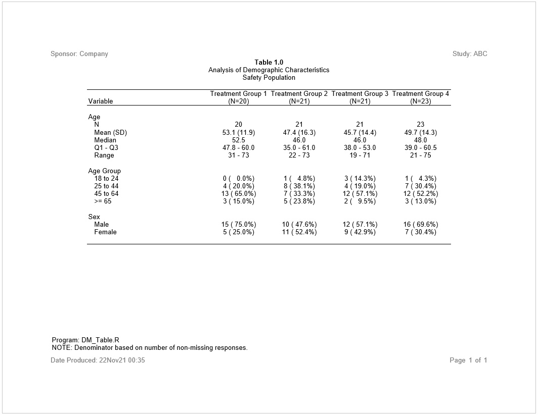
Log
Here is the log produced by the above sample program:
=========================================================================
Log Path: C:/Users/dbosa/AppData/Local/Temp/RtmpcV9Bys/log/example1.log
Program Path: C:\packages\Testing\fmtr_example1.R
Working Directory: C:/packages/Testing
User Name: dbosa
R Version: 4.1.2 (2021-11-01)
Machine: SOCRATES x86-64
Operating System: Windows 10 x64 build 19041
Base Packages: stats graphics grDevices utils datasets methods base
Other Packages: tidylog_1.0.2 reporter_1.2.6 libr_1.2.1 fmtr_1.5.3 logr_1.2.7
                sassy_1.0.5 forcats_0.5.1 stringr_1.4.0 dplyr_1.0.7 purrr_0.3.4
                readr_2.0.2 tidyr_1.1.4 tibble_3.1.5 ggplot2_3.3.5 tidyverse_1.3.1
Log Start Time: 2021-11-17 10:32:36
=========================================================================

=========================================================================
Prepare Data
=========================================================================

# library 'sdtm': 1 items
- attributes: csv not loaded
- path: C:/Users/dbosa/Documents/R/win-library/4.1/fmtr/extdata
- items:
  Name Extension Rows Cols    Size        LastModified
1   DM       csv   87   24 45.4 Kb 2021-11-16 10:34:25

lib_load: library 'sdtm' loaded

select: dropped 20 variables (STUDYID, DOMAIN, SUBJID, RFSTDTC, RFENDTC, <U+0085>)

filter: removed 2 rows (2%), 85 rows remaining

# A tibble: 85 x 4
   USUBJID    SEX     AGE ARM
   <chr>      <chr> <dbl> <chr>
 1 ABC-01-049 M        39 ARM D
 2 ABC-01-050 M        47 ARM B
 3 ABC-01-051 M        34 ARM A
 4 ABC-01-052 F        45 ARM C
 5 ABC-01-053 F        26 ARM B
 6 ABC-01-054 M        44 ARM D
 7 ABC-01-055 F        47 ARM C
 8 ABC-01-056 M        31 ARM A
 9 ABC-01-113 M        74 ARM D
10 ABC-01-114 F        72 ARM B
# ... with 75 more rows

Get ARM population counts

count: now 4 rows and 2 columns, ungrouped

ARM A ARM B ARM C ARM D
   20    21    21    23

=========================================================================
Create format catalog
=========================================================================

# A format catalog: 3 formats
- $AGECAT: type U, 5 conditions
- $SEX: type U, 4 conditions
- $VAR: type V, 3 elements

=========================================================================
Create summary statistics for age
=========================================================================

group_by: one grouping variable (ARM)

summarise: now 4 rows and 6 columns, ungrouped

pivot_longer: reorganized (N, Mean (SD), Median, Q1 - Q3, Range) into (label, value) [was 4x6, now 20x3]

pivot_wider: reorganized (ARM, value) into (ARM A, ARM B, ARM C, ARM D) [was 20x3, now 5x5]

# A tibble: 5 x 6
  var   label     `ARM A`     `ARM B`     `ARM C`     `ARM D`
  <chr> <chr>     <chr>       <chr>       <chr>       <chr>
1 AGE   N         20          21          21          23
2 AGE   Mean (SD) 53.1 (11.9) 47.4 (16.3) 45.7 (14.4) 49.7 (14.3)
3 AGE   Median    52.5        46.0        46.0        48.0
4 AGE   Q1 - Q3   47.8 - 60.0 35.0 - 61.0 38.0 - 53.0 39.0 - 60.5
5 AGE   Range     31 - 73     22 - 73     19 - 71     21 - 75

=========================================================================
Create frequency counts for Age Group
=========================================================================

Create age group frequency counts

mutate: new variable 'AGECAT' (character) with 4 unique values and 0% NA

select: dropped 3 variables (USUBJID, SEX, AGE)

group_by: 2 grouping variables (ARM, AGECAT)

summarize: now 15 rows and 3 columns, one group variable remaining (ARM)

pivot_wider: reorganized (ARM, n) into (ARM A, ARM B, ARM C, ARM D) [was 15x3, now 4x5]

transmute: dropped one variable (AGECAT)

           new variable 'var' (character) with one unique value and 0% NA

           new variable 'label' (factor) with 4 unique values and 0% NA

           converted 'ARM A' from integer to character (0 new NA)

           converted 'ARM B' from integer to character (0 new NA)

           converted 'ARM C' from integer to character (0 new NA)

           converted 'ARM D' from integer to character (0 new NA)

# A tibble: 4 x 6
  var    label    `ARM A`     `ARM B`    `ARM C`     `ARM D`
  <chr>  <fct>    <chr>       <chr>      <chr>       <chr>
1 AGECAT 18 to 24 0 (  0.0%)  1 (  4.8%) 3 ( 14.3%)  1 (  4.3%)
2 AGECAT 25 to 44 4 ( 20.0%)  8 ( 38.1%) 4 ( 19.0%)  7 ( 30.4%)
3 AGECAT 45 to 64 13 ( 65.0%) 7 ( 33.3%) 12 ( 57.1%) 12 ( 52.2%)
4 AGECAT >= 65    3 ( 15.0%)  5 ( 23.8%) 2 (  9.5%)  3 ( 13.0%)

=========================================================================
Create frequency counts for SEX
=========================================================================

select: dropped 2 variables (USUBJID, AGE)

group_by: 2 grouping variables (ARM, SEX)

summarize: now 8 rows and 3 columns, one group variable remaining (ARM)

pivot_wider: reorganized (ARM, n) into (ARM A, ARM B, ARM C, ARM D) [was 8x3, now 2x5]

transmute: dropped one variable (SEX)

           new variable 'var' (character) with one unique value and 0% NA

           new variable 'label' (factor) with 2 unique values and 0% NA

           converted 'ARM A' from integer to character (0 new NA)

           converted 'ARM B' from integer to character (0 new NA)

           converted 'ARM C' from integer to character (0 new NA)

           converted 'ARM D' from integer to character (0 new NA)

mutate: converted 'label' from factor to character (0 new NA)

# A tibble: 2 x 6
  var   label  `ARM A`     `ARM B`     `ARM C`     `ARM D`
  <chr> <chr>  <chr>       <chr>       <chr>       <chr>
1 SEX   Male   15 ( 75.0%) 10 ( 47.6%) 12 ( 57.1%) 16 ( 69.6%)
2 SEX   Female 5 ( 25.0%)  11 ( 52.4%) 9 ( 42.9%)  7 ( 30.4%)

Combine blocks into final data frame

# A tibble: 11 x 6
   var    label     `ARM A`     `ARM B`     `ARM C`     `ARM D`
   <chr>  <chr>     <chr>       <chr>       <chr>       <chr>
 1 AGE    N         20          21          21          23
 2 AGE    Mean (SD) 53.1 (11.9) 47.4 (16.3) 45.7 (14.4) 49.7 (14.3)
 3 AGE    Median    52.5        46.0        46.0        48.0
 4 AGE    Q1 - Q3   47.8 - 60.0 35.0 - 61.0 38.0 - 53.0 39.0 - 60.5
 5 AGE    Range     31 - 73     22 - 73     19 - 71     21 - 75
 6 AGECAT 18 to 24  0 (  0.0%)  1 (  4.8%)  3 ( 14.3%)  1 (  4.3%)
 7 AGECAT 25 to 44  4 ( 20.0%)  8 ( 38.1%)  4 ( 19.0%)  7 ( 30.4%)
 8 AGECAT 45 to 64  13 ( 65.0%) 7 ( 33.3%)  12 ( 57.1%) 12 ( 52.2%)
 9 AGECAT >= 65     3 ( 15.0%)  5 ( 23.8%)  2 (  9.5%)  3 ( 13.0%)
10 SEX    Male      15 ( 75.0%) 10 ( 47.6%) 12 ( 57.1%) 16 ( 69.6%)
11 SEX    Female    5 ( 25.0%)  11 ( 52.4%) 9 ( 42.9%)  7 ( 30.4%)

=========================================================================
Create and print report
=========================================================================

# A report specification: 1 pages
- file_path: 'output/example1.rtf'
- output_type: RTF
- units: inches
- orientation: landscape
- margins: top 1 bottom 1 left 1 right 1
- line size/count: 9/40
- page_header: left=Sponsor: Company right=Study: ABC
- title 1: 'Table 1.0'
- title 2: 'Analysis of Demographic Characteristics'
- title 3: 'Safety Population'
- footnote 1: 'Program: DM_Table.R'
- footnote 2: 'NOTE: Denominator based on number of non-missing responses.'
- page_footer: left=Date Produced: 17Nov21 10:32 center= right=Page [pg] of [tpg]
- content:
# A table specification:
- data: tibble 'final' 11 rows 6 cols
- show_cols: all
- use_attributes: all
- stub: var label 'Variable' width=2.5 align='left'
- define: var 'Variable' dedupe='TRUE'
- define: label 'Demographic Category'
- define: ARM A 'Treatment Group 1'
- define: ARM B 'Treatment Group 2'
- define: ARM C 'Treatment Group 3'
- define: ARM D 'Treatment Group 4'

=========================================================================
Clean Up
=========================================================================

lib_sync: synchronized data in library 'sdtm'

lib_unload: library 'sdtm' unloaded

=========================================================================
Log End Time: 2021-11-17 10:32:36
Log Elapsed Time: 0 00:00:00
=========================================================================